
overviewPreface
Today we continue with the new TSMaster feature - MATLAB Automation Control Module. This module provides a large number of widgets for MBD development. Also included is this program that automatically converts c code to stateflow code.
I. MATLAB's automation objects
MATLAB automation object
> First click on Connect to connect to the matlab automation object, you need to start the main program of matlab, once connected, the matlab program can be controlled by the TSMaster software in real time. Then after we click on it we can see that the Connect button is grayed out and then the Disconnect button is highlighted, then the matlab program can be controlled by our software at this time.

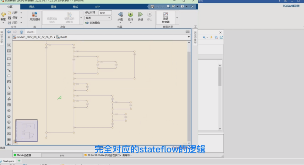
> Then we can click this c code to stateflow, click parse, will realize a logic tree, and then click generate code. At this time we can see that our sample code can be automatically converted to stateflow code, the function can quickly convert the existing C code logic into a completely equivalent stateflow logic, thus improving the development efficiency of MBD. Then the effect of the conversion is completed is this, double-click the chart1 to expand after you can see with the C script just corresponding to the logic of the stateflow.
II. Automated construction of SIL and HIL environments
Automatic build of SIL and HIL
As long as we have a simulation model of Simulink that can generate code, we can use this module to realize the real-time operation of this model in the TSMaster environment. Thus our algorithms can be involved in the real-time simulation of HIL and SIL in the early stage of software design. Meanwhile, with the support of the applet, we can also debug and monitor the algorithms in a detailed way, and even release the binary files to other users for co-simulation, so how do we realize it?
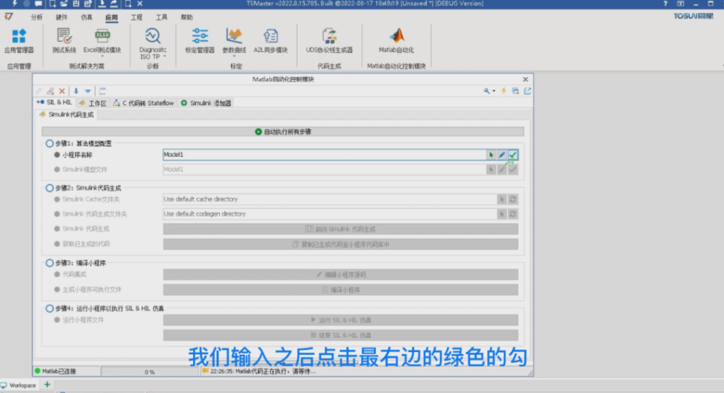
> Let's start from 0 and give an example to illustrate: first we switch to the first page, the SIL and HIL page, we can see that this page has 4 steps, according to the sequence of the execution of these 4 steps, you can quickly build a HIL environment. So the first step is the configuration of the algorithm model, he gave two inputs, one is the name of our applet, the second is the Simulink model file. For the first input, just give us a name for the newly constructed applet, for example, the default Model1, we input and click on the green tick on the right side, its function is to determine whether Model1 exists. If it doesn't exist, create one, if it does, use this Model1.
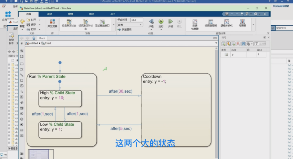
> This allows us to integrate our new algorithm into our existing applet, where it is necessary to fill in the model name of the existing applet, that is, from which we can choose the name of our applet. Then after this step, we come to the process of setting up the Simulink model file. Here we need to find a Simulink example program to explain, we first open Simulink, in the Simulink start page will have a lot of examples. We look for an example to expand this stateflow, which has a blank map, simple map layered map and so on. We choose this layered diagram, it opens a model named untitled, we see this model, contains a run and a cooldown. these two big state run after 30 seconds, will cool down 5 seconds, and then after 5 seconds to continue to run, and from then on the cycle repeats, and in the process of this run, is every 1 second to let the output between 10 and 1 This is the simple logic of the current stateflow.
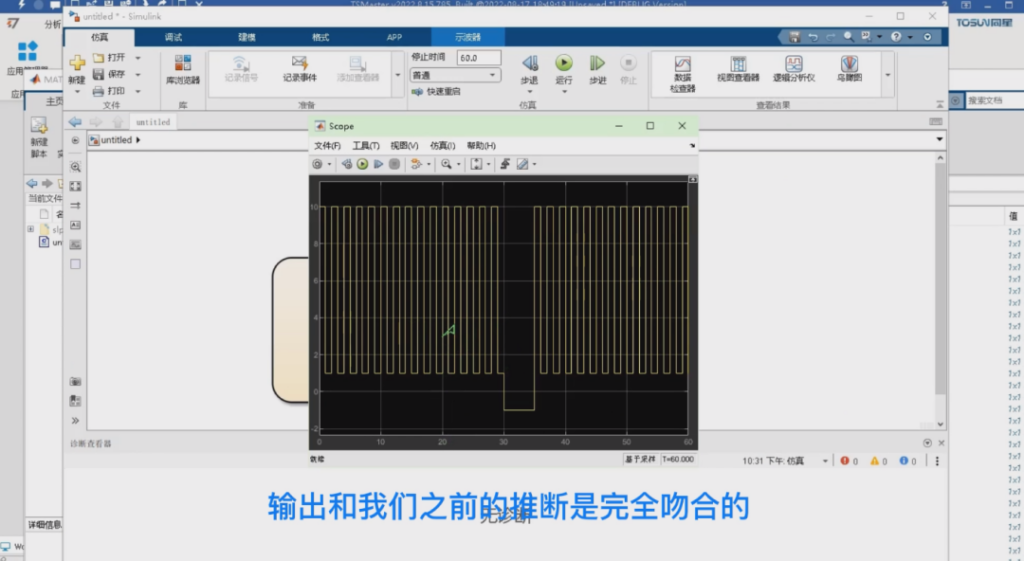
> Press esc to go back to the top level, we can see that there is only one output in this model, let's add an oscilloscope to see the waveform. Press F5 to run, of course, this run needs to switch off the current working directory, we can choose any directory, such as a new folder, and then we go back to the model just now and press F5 to run successfully, then open the oscilloscope we can see that the output and our previous inference is exactly the same. That is to say, after running for 30 seconds, we will take a break for 5 seconds and then continue to run. We save the model as simple, then delete the oscilloscope and add an out interface to configure the model for code generation, then we have to configure the details of code generation.
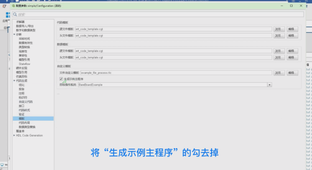
> We enter the model settings, click on the code generation, first of all, we need to change this grt to ert.tlc, because the target environment is an embedded environment, and check the box to generate code only, and then expand the code generation, go to the template, remove the check box "Generate sample main program", so that it will not automatically generate the main function. function. Because the main function of the file is often not used. The configuration is now complete. We click Save and close the model.
III. MATLAB control module
MATLAB Control module
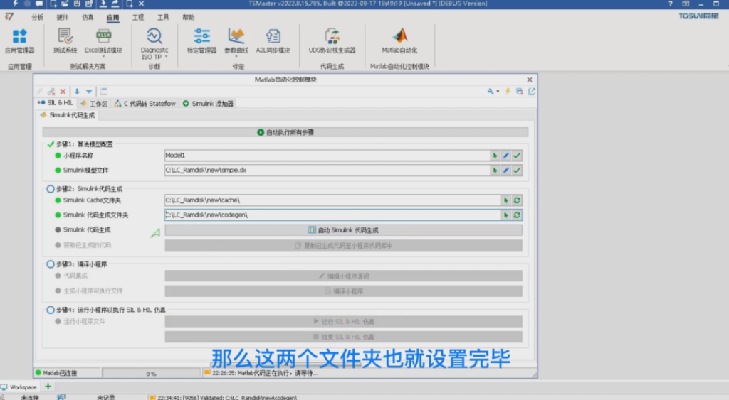
> Next, go back to the matlab control module, select the Simulink model file, click the green arrow button, select the simple.slx, then you can see that after the first two steps, step 1 is completed. The next step is to set the cache folder and codegen folder, then leave them empty to indicate that they are generated to the default location. We can change these two locations, or click the green button, and then you can select our cache folder, we can create a new cache, and select this folder, then the cache folder has been set successfully. Next is codegen, still the same, we can create a codegen next to cache, click to select it, then these two folders have been set up.
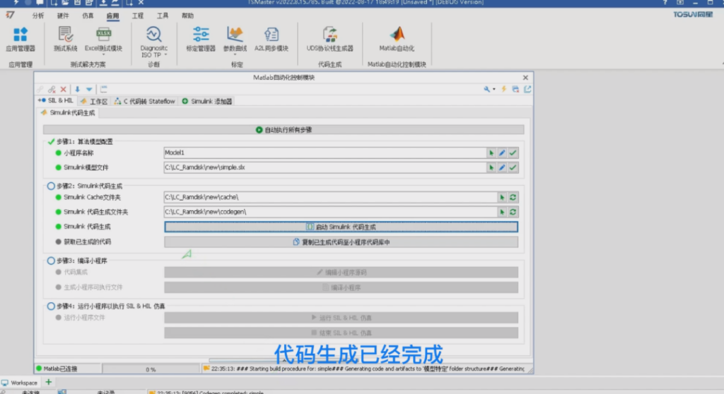
> Then it's time for code generation. We just have to click on Start Simulink Code Generation and wait for the code generation to finish. Then the generated code will be stored in the codegen folder that we have just set. The first generation will take a little bit of time, so we need to be patient. Then the Simulink execution process is synchronized and slower, so TSMaster may alarm. Now we can see that the code generation is finished.
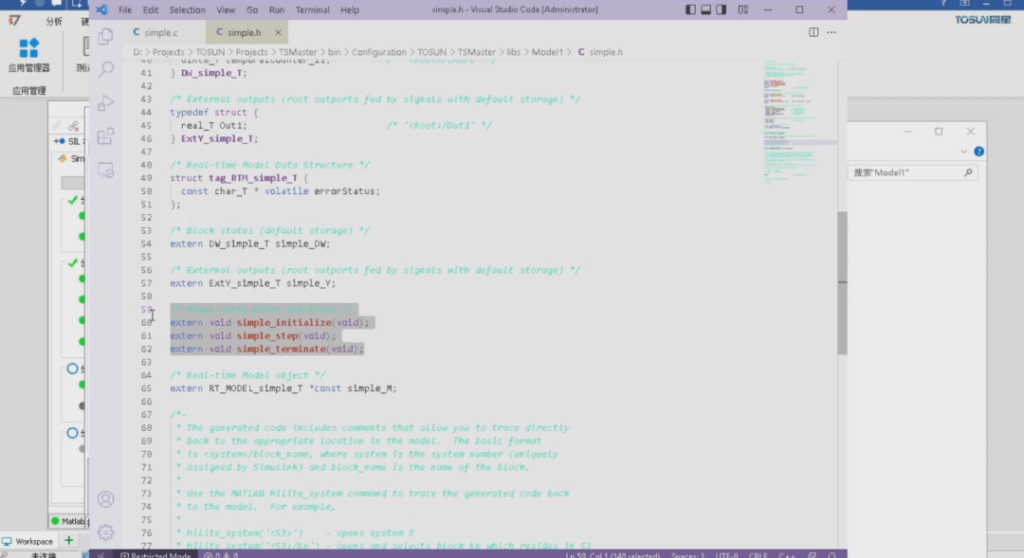
> Then the next step is to automatically copy the generated code to the code base of our small program, after clicking can be shown to have copied 6 files, then the next step has been completed. That is, the code generation process has been successfully realized, and then the next is code integration. The purpose of code integration is to call the algorithm, we click on the source code button to edit the program, open the Model1 program, we first look at the properties, and then click on the path of the code base, you can see the simple.c and .h files and some other header files used. Open these two files, first we look at the simple.h file, then this file is an interface file, you can see that there are three functions, initialization step and terminate function, we need to copy these three function calls to the Model1 applet. The first thing is to use this simple.h header file.
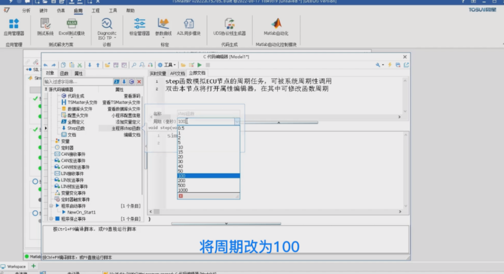
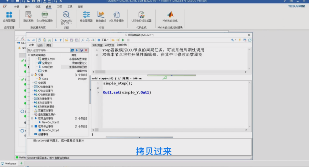
> We go back to our applet and click on global definition #include, "simple.h". Then the next is COPY. we double-click this simple initialization, and then to the initialization event of the applet, paste and then COPY STEP to our applet's STEP function, paste and then TERMINATE, back to our applet's STOP event, the same paste, so as to achieve the function call. Then we need to pay attention to the period of the step function, the default period is 5 milliseconds, but the model is certainly not. Let's start by opening up this simple.slx, and then we'll go to the properties of the model and look at the properties of the solver associated with the model. It's a fixed step size, and the step size is 0.1 seconds, so 0.1 seconds is 100 milliseconds in TSMaster, double-click on the STEP function, change the period to 100, and then the next thing we need to do is to observe the signal out1.
> We can directly in the variable point right click, add variable, enter us this out1, then a new out1 variable, then we need to find this variable in the code, then you can see this extern, here is written outports, that is, simple y this variable, it has a member called out1, that is, we need to use the variable, we can write out1.set here to copy this out1 just now, so that we can realize the assignment of the variable. Then the program is finished.
IV. Execution of HIL and SIL simulations
Perform emulation of HIL and SIL
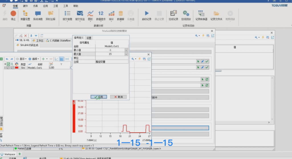
> Here we can directly click to run the simulation, then our algorithm model has been running in real time, at this time if you need to observe the signal, first of all, we need to start our TSMaster simulation, and then we can open an observation window, such as the graph, after the opening we can click the right button to add the system variables, through the internal variables, to find out 1 model 1 out 1 this variable, then we can modify his range, for example, change to 1-15 -1-15, then we can see the graph display exactly the same as we just saw Simulink oscilloscope screen. This variable, then we can modify his range, for example, changed to 1-15 -1-15, then you can see the graphic display and we just saw the Simulink oscilloscope screen is exactly the same.
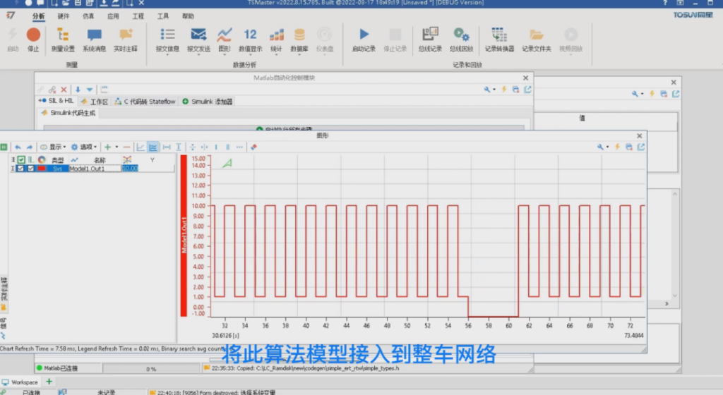
> This signal can be set as a vertical line display, which is more in line with the logical meaning of this signal represents, then this out1 signal is real-time refresh, which means that we can access this algorithmic model through the bus interface to the entire vehicle network, you can interact with the actual controller, then the above is the matlab control module for HIL in a simple way.
About More
This is the new features of TSMaster MATLAB automation control module, we will see you in the next issue! (You can watch our B-site video for specific operation explanation)


